
What is Crypto Algorithmic Trading? (Crypto Algo Trading)
Crypto algorithmic trading is the use of automations to execute cryptocurrency trades to capitalize on market opportunities efficiently. Trading algorithms analyze market and historical data, blend statistical models and predefined criteria to trade cryptocurrencies.
Crypto algo trading may involve machine learning techniques, which trains the algorithm to evolve with the market and new data inputs. Some common machine learning techniques include decision trees, support vector machines and artificial neural networks (ANNs).
In today’s guide, we’ll be covering how to develop a crypto trading algorithm using an artificial neural network, using the Open High Low Close Volume (OHLCV) endpoint from the GeckoTerminal API.
Artificial Neural Networks in Crypto Algorithmic Trading
Artificial neural networks are computational models that simulate human decision-making, whereby it is capable of learning and adapting based on its environment and new data inputs. In the context of crypto trading, an ANN functions as a trader continuously monitoring asset prices 24/7, adapting trading positions based on historical and live data, among other metrics.
This can be achieved as ANNs comprise layers of interconnected nodes and process information through weighted connections – as such, it is able to learn and recognize complex data patterns.ANNs can therefore be employed for predictive analysis and decision-making in executing crypto trades. They analyze historical market data, identify patterns, and adjust trading strategies based on evolving market conditions.
Understanding Input, Hidden and Output Layers
It is important to understand how the ANN’s interconnected nodes are divided into three layers and its corresponding statistical representation, as these will be covered in scripts later on.
-
Input layer – Independent variables
The input layer, which corresponds to independent variables, serves as the entry point for data into the neural network. -
Hidden layer – Coefficient (weights)
The hidden layer is associated with coefficients or weights. These weights are adjusted during the processing of input data to optimize the network's performance. -
Output layer – Dependent variable
The output layer is linked to the dependent variable, where the final result or prediction is produced, based on the information processed.
How it comes together: Inputs are fed into the model to be processed (i.e. summed). If the result of this summation is a value that exceeds the threshold, the node adjusts the weight matrices. The process of adjustment is known as ‘training’ a neural network, and the most common feedback method to perform these amendments is called backpropagation. Without this algorithm, we would have to identify the impact each weight has on the model's error and update each individual coefficient. Instead, the error is fed back (back propagated) into the network, progressing one layer at a time until it is minimized in the model. This creates a trained ANN that can continue to analyze data.
Prerequisites: Python Libraries & Importing OHLC Data
Before we dive into the crypto trading algorithms, we will first need to import the following python libraries to extract our dataset from the GeckoTerminal API and build it into a legible dataframe. The pandas library is useful to visualize and manipulate our data in a legible dataframe. The numpy package is practical when dealing with arrays and different functions, and the matplotlib.pyplot library can be used to visualize our strategies results.
import pandas as pd
import numpy as np
import matplotlib.pyplot as plt
import requests

from datetime import datetime, timedelta
After this, we will import our data into our integrated development environment (IDE) – for this demo, I’ve used Visual Studio, and followed the same process outlined in my previous article on using Python to parse CoinGecko API.
We will now import Ethereum network data from the DAI-WETH pool, between the time period of August 23, 2023 to December 30, 2023.
# Import data from GeckoTerminal DEX API
network = 'eth'
pool_address = '0x60594a405d53811d3bc4766596efd80fd545a270' #DAI-WETH Pool
parameters = f'{network}/pools/{pool_address}'
specificity = f'{1}'
#URL with your specifications
url = f'https://api.geckoterminal.com/api/v2/networks/{parameters}/ohlcv/day?aggregate={specificity}'
response = requests.get(url)
data = response.json()
#Turning into pandas dataframe, turning the date value into datetime format, making it the index
data = data['data']['attributes']['ohlcv_list']
df = pd.DataFrame(data, columns=['Date', 'Open', 'Close', 'High', 'Low', 'Volume'])
df['Date'] = pd.to_datetime(df['Date'], unit = 's')
df.set_index('Date', inplace = True)
df
This returns a clear and legible dataset that includes the DAI-WETH OHLC price on the UniSwap exchange, alongside its volume. Additionally, the ‘date’ each price was quoted is now the index.
| Open | Close | High | Low | Volume | |
| 2023-11-30 | 0.998109 | 1.008865 | 0.996222 | 0.999061 | 1.44E+06 |
| 2023-11-29 | 1.001466 | 1.006282 | 0.987182 | 0.998109 | 5.72E+06 |
| 2023-11-28 | 0.997525 | 1.006695 | 0.996104 | 1.001466 | 6.33E+06 |
| 2023-11-27 | 1.001736 | 1.005328 | 0.99297 | 0.997525 | 1.03E+07 |
| 2023-11-26 | 0.996809 | 1.003089 | 0.995526 | 1.001736 | 3.33E+06 |
| ... | ... | ... | ... | ... | ... |
| 2023-08-27 | 1.001585 | 1.002673 | 0.9968 | 0.998802 | 1.54E+06 |
| 2023-08-26 | 0.998725 | 1.003637 | 0.997711 | 1.001585 | 1.17E+06 |
| 2023-08-25 | 0.999884 | 1.036346 | 0.988577 | 0.998725 | 7.69E+06 |
| 2023-08-24 | 0.998746 | 1.142734 | 0.958476 | 0.999884 | 9.25E+06 |
| 2023-08-23 | 0.999344 | 1.01471 | 0.994517 | 0.998746 | 7.78E+06 |
100 rows × 5 columns
Specifically for developing artificial neural networks, we will also require the following two python libraries:
- Tensorflow: Tensorflow is a machine learning (ML) library that provides the core functionality for training neural networks.
- Keras: Keras is a high-level python neural network API, which allows developers to exercise complex functionalities without having to deal with granularities. With pre-built functions and modules for common tasks, it enables developers to express their code in a more human-readable manner.
💡Pro-tip: Instead of manually defining the operations for each layer, Keras allows us to specify the design of our ANN in a clear and legible syntax.
# Creating ANN Model
import tensorflow.python.tools
from tensorflow.keras.models import Sequential
from tensorflow.keras.layers import Dense, Dropout
layer_builder = Sequential()
The ‘Sequential’ class at the bottom of the above quote, initiated as ‘layer_builder’, is a part of the Keras API within Tensorflow. It allows us to add layers to our ANN one at a time, in a layer-by-layer fashion. The Dense layer is a fully connected layer that links each neuron in a layer to every neuron in the next layer. Lastly, the Dropout layer is used to prevent overfitting. During training, it randomly drops out a fraction of inputs, which helps prevent the network from overlying on certain nodes and encourages more robust learning.
Training the ANN with Crypto Price Data
We will need to train our ANN in order to build our crypto algorithmic trading strategy. We’ll employ the following 3 basic technical analysis techniques to train our ANN:
- 3-month moving average (3MA)
- 10-month moving average (10MA)
- 15-month moving average (15MA)
The output value is binary (defined as 1 or 0), varying when the price rises or falls between periods (hence the new df[‘Price_Rise’] column). These measurements are stored in our dataframe as new columns. Our X data thus includes all rows and the 6th to N-1th column (i.e. ‘3MA’ to ‘15MA’). Our Y data is all the rows in the ‘Price_Rise’ column (which is the last column).
# Clean up and standardize data
df['3MA'] = df['Close'].shift(1).rolling(window = 3).mean()
df['10MA'] = df['Close'].shift(1).rolling(window = 10).mean()
df['15MA'] = df['Close'].shift(1).rolling(window = 15).mean()
df['Price_Rise'] = np.where(df['Close'].shift(-1) > df['Close'], 1, 0)
df = df.dropna()
X = df.iloc[:, 5:-1]
Y = df.iloc[:, -1]
The objective here is to split up our X data (i.e. 3MA, 10MA, and 15MA columns) and the Y dataset (i.e. price rise or fall) into training and testing sets.
The training set is used to arrive at the adjusted weights through backpropagation, while the test set is used to see how the model would perform on newly instituted data, which is our backtest. After using the test data set, we will employ several metrics to determine the efficiency of our model.
#Create X_train, X_test, Y_train, Y_test
split_data = int(len(df)*0.7)
X_train, X_test, Y_train, Y_test = X.iloc[:split_data, :], X.iloc[split_data:, :], Y.iloc[:split_data], Y.iloc[split_data:]
Standardizing the Dataset
Standardizing the dataset is a crucial step because it will ensure the mean of our inputs is 0 and the standard deviation is 1. This therefore confirms the data is unbiased, due to the varying scales of our inputs.
💡Pro-tip: Neglecting this step of standardizing the dataset may result in the model “over-weighing” features with higher average returns, and is not recommended.
The StandardScaler class from sklearn facilitates this process, as it removes the mean and scales to unit (=1) variance. ‘Scaler’ is created as an instance of StandardScaler. The ‘fit_transform’ method fits to the training set data (X_train) and calculates its mean and standard deviation. The ‘transform’ method uses the mean and standard deviation calculated from the training set to standardize the test set (X_test). As the Y_train and Y_test are binary values—from price increasing or decreasing—we do not need to apply the same standardizing methods.
#Standardize Data
from sklearn.preprocessing import StandardScaler
scaler = StandardScaler()
X_train = scaler.fit_transform(X_train)
X_test = scaler.transform(X_test)
Adding Layers
We will now proceed with creating our linear stack of layers.
For our first densely connected layer, we create ‘128’ neurons for our hidden layer, which, as the name prescribes, is hidden.
The activation function ‘relu’ abbreviates Rectified Linear Unit. A popular choice for the activation function, ‘relu’ introduces non-linearity to the neural network. This causes the ANN to learn and represent more complex and non-linear relationships in the data.
‘Input_dim’ simply determines the dimensions of our inputs. We set this to be the exact shape of our X data by using the ‘shape()’ function in numpy.
After building several layers, we construct our output layer, which includes one node as we require one output. Additionally, we use the ‘sigmoid’ function because it returns values between 0 and 1, as it represents the probability of the market moving favorably.
# First input layer
layer_builder.add(Dense(units = 128, kernel_initializer = 'uniform',
activation = 'relu', input_dim = X.shape[1]))
# Second input layer
layer_builder.add(Dense(units = 128, kernel_initializer = 'uniform'
, activation = 'relu'))
# Output layer
layer_builder.add(Dense(units = 1, kernel_initializer = 'uniform', activation = 'sigmoid'))
Improving Predictive Capabilities
Our goal is to improve the predictive capabilities of the ANN and minimize the difference (also known as ‘the residual’) between predicted and observed data. This is commonly done through a process called ‘gradient descent’. This method minimizes the ‘cost function’, which is a function of the cost of making a prediction using the neural network. It is a measure of how far off the predicted value, y^, is from the actual value, y.
While there are many cost functions used in practice, we will aim to minimize the ‘mean_squared_error’ which is the squared sum of our residuals, divided by the number of observations:
-
SSR = Σᵢ(𝑦ᵢ − 𝑓(𝐱ᵢ))² for all observations 𝑖 = 1, …, 𝑛, where 𝑛 is the total number of observations.
-
MSE = SSR / 𝑛
-
The measurement of our success (‘metrics’) is set to ‘accuracy’, which calculates how often our predictions were correct.
We will use ‘adam’ to optimize when compiling our layers, as it is computationally efficient and requires little memory usage. Adam is an optimization algorithm that we can use instead of the classical stochastic gradient descent procedure to update our neural network weights. It is straightforward to implement, making it a good starting point for building ANNs.
# Compile the layers
layer_builder.compile(optimizer = 'adam', loss = 'mean_squared_error', metrics = ['accuracy'])
We then fit our ANN to our training data, using a ‘batch size’ of 5, which is the number of data points used to compute the error before backpropagation, and 100 ‘epochs’, the number of times the training model will be used on the training set.
The keras ‘predict’ method generates output predictions given our input data ‘X_test’. We then obtain a binary variable by defining Y_pred as true when it is greater than 0.5, and false when it is less.
#Fit ANN to training set
layer_builder.fit(X_train, Y_train, batch_size = 5, epochs = 100)
Y_pred = layer_builder.predict(X_test)
Y_pred = (Y_pred > 0.5)
#Store predictions back into dataframe
df['Y_Pred'] = np.NaN
df.iloc[(-len(Y_pred)):,-1:] = Y_pred.flatten()
#Fit ANN to training set
layer_builder.fit(X_train, Y_train, batch_size = 5, epochs = 100)
Y_pred = layer_builder.predict(X_test)
Y_pred = (Y_pred > 0.5)
#Store predictions back into dataframe
df['Y_Pred'] = np.NaN
df.iloc[(-len(Y_pred)):,-1:] = Y_pred.flatten()
Visualizing the Returns
We can compute and visualize our price returns based on our crypto trading strategy, through the following code. This outputs a log-return visualization of our ANN, relative to the performance of simply holding Ethereum.
# Strategy Returns
df['Returns'] = 0
# Get the log returns
df['Returns'] = np.log(df['Close']/df['Close'].shift(1))
# Shift so that the returns are in line with the day they were achieved
df['Returns'] = df['Returns'].shift(-1)
df['Strategy Returns'] = 0
df['Strategy Returns'] = np.where(df['Y_Pred'] == True, df['Returns'], - df['Returns'])
df['Cumulative Market Returns'] = np.cumsum(df['Returns'])
df['Cumulative Strategy Returns'] = np.cumsum(df['Strategy Returns'])
# Visualize Returns
plt.figure(figsize=(12,4))
plt.plot(df['Cumulative Strategy Returns'], color = 'Blue', label = 'Strategy Returns')
plt.plot(df['Cumulative Market Returns'], color = 'Green', label = 'Market Returns')
plt.xlabel('Date')
plt.xticks(df.index[::5], rotation = 45)
plt.ylabel('Log-Returns')
plt.legend()
plt.show()
As a result of the code, we see the following chart:
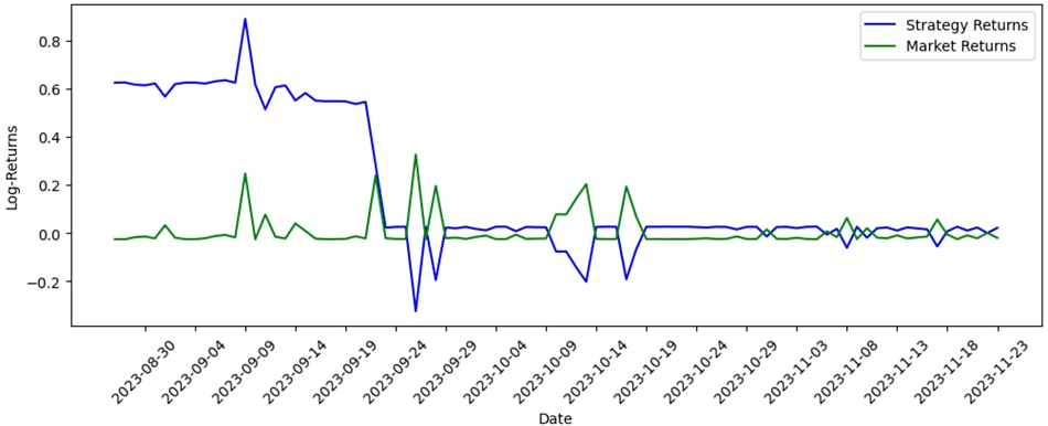
Analyzing the data visualization, we can see that there are exorbitantly high returns in the first 15 days, followed by an interestingly negative relationship between the strategy and market returns share, over the next few months. This issue could stem from overfitting; excessive reliance on the training data set may lead to initially high returns. We should therefore acquire more data for the training and testing sets – as with all machine learning models, this crypto trading algorithm has the potential to be improved with more data points and larger data sizes, which would enhance the training and development of the ANN.
To wrap up, in this demo we have created a crypto trading algorithm capable of forward feeding and back-propagating, creating predictions off 3-, 10- and 15-day moving averages. These predictions are then back-tested against monthly price data, allowing us to compare it to the performance of simply holding Ethereum.
For Advanced Traders: Build Your Own Crypto Trading Algorithm with Richer Crypto Data
GeckoTerminal’s DEX data API is currently publicly accessible in beta and will soon be integrated into CoinGecko API. Some of the most popular endpoints include:
- OHLCV data, as covered in this guide
- Trending liquidity pools on a network
- Top liquidity pools for a token, and more!
To avoid getting rate limited, advanced traders can consider subscribing to our Analyst API plan and will be extended a GeckoTerminal API key upon request.

Interested in more API or trading-related resources? This extensive DEX Data API guide will walk you through how to get market data for a liquidity pool, access on-chain data for DEX-traded tokens and more!


 Or check it out in the app stores

